
| 일 | 월 | 화 | 수 | 목 | 금 | 토 |
|---|---|---|---|---|---|---|
| 1 | 2 | 3 | ||||
| 4 | 5 | 6 | 7 | 8 | 9 | 10 |
| 11 | 12 | 13 | 14 | 15 | 16 | 17 |
| 18 | 19 | 20 | 21 | 22 | 23 | 24 |
| 25 | 26 | 27 | 28 | 29 | 30 | 31 |
- dp
- manganinja
- posco 채용
- 과제형 코딩테스트
- controlNet
- diffusion models
- DDPM
- kt인적성
- ddim
- 포스코 채용
- Generative Models
- 프로그래머스
- Image Generation
- 논문 리뷰
- KT
- stable diffusion
- classifier-free guidance
- ip-adapter
- colorization
- 포스코 코딩테스트
- 코딩테스트
- Today
- Total
Paul's Grit
[논문 리뷰] [DDPM] Denoising Diffusion Probabilistic Models 본문
[논문 리뷰] [DDPM] Denoising Diffusion Probabilistic Models
Paul-K 2024. 5. 14. 22:37Jonathan Ho, Ajay Jain, Pieter Abbeel
UC Berkeley
NeurIPS 2020 [Paper]
1. Introduction
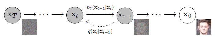
Diffusion Probabilistic Models (이하 Diffusion Models)에는 forward process와 reverse process가 있다.
그림에서처럼 forward process는 image to noise, reverse process는 noise to image의 과정이다.
이때, 딥러닝에 의해 paramieterize되는 부분은 reverse process이다.
2. Background
2.1 Forward (Diffusion) Process
본 논문에서 Diffusion process $q(x_{1:T}|x_{0})$는 Marchov chain으로 data에 Gaussian noise ($\epsilon \sim \mathcal{N}(0, 1)$)를 추가하는 과정이다. $q(x_{1:T}|x_{0})$를 forward process posteriors 또는 approximate posterior라고 부르기도 한다.
참고: Marchov chain은 마르코프 성질, "과거와 현재 상태가 주어졌을 때의 미래 상태의 조건부 확률 분포가 과거 상태와는 독립적으로 현재 상태에 의해서만 결정됨", 을 가진 이산 확률 과정.
What distinguishes diffusion models from other types of latent variable models is that the approximate posterior $q(x_{1:T}|x_{0})$, called the forward process or diffusion process, is fixed to a Markov chain that gradually adds Gaussian noise to the data according to a variance schedule $\beta_1, \cdots , \beta_T$:

가우시안 노이즈를 추가해주는 과정은 $X_{t-1}$을 $\sqrt{1-\beta_t}$ 만큼 누그러뜨리고, $\sqrt{\beta_t}\epsilon$ 만큼 더해주는 방식으로 진행된다.
$X_t = \sqrt{1-\beta_t}X_{t-1} + \sqrt{\beta_t}\epsilon $의 형태를 취한 이유는 $X_t$의 분산이 매 time step마다 1을 유지하고, 최종적으로 $\mathcal{N}(0,1)$에 도달하기 위함이라고 한다.
뒤에서 설명되겠지만, $\beta_t$를 상수로 고정함으로써 forward precess는 학습되는 parameters를 가지지 않는다.
$\beta_{t}$는 사전에 정의된 값이고, 뒤로 갈 수록 커진다. 실험파트에서 설명되는데, $T=1000$이고, $\beta_1=10^{-4}$에서 $\beta_T=0.02$로 linear하게 증가시켰다고 한다.
Forward (diffution) process의 유용한 점은 $q(X_t|X_0)$ 을 $X_t = \sqrt{\bar{\alpha}_t}X_0+\sqrt{1-\bar{\alpha}_t}\epsilon, \epsilon \sim \mathcal{N}(0,1)$와 같이 한번에 구할 수 있다는 점이다.
A notable property of the forward process is that it admits sampling $x_t$ at an arbitrary timestep $t$ in closed form: using the notation $ \alpha_t := 1 - \beta_t$ and $\bar{\alpha}_t:=\prod_{s=1}^{t}\alpha_s$, we have

2.2 Reverse (Denoising) process
Diffusion models are latent variable models of the form $p_{\theta}(x_0) := \int p_{\theta}(x_{0:T})dx_{1:T}$, where $x_1, \cdots, x_T$ are latents of the same dimensionality as the data $x_0 \sim q(x_0)$. The joint distribution $p_{\theta}(x_{0:T})$ is called the $\textit{reverse process}$, and it is defined as a Markov chain with learned Gaussian transitions starting at $p(x_T ) = \mathcal{N}(x_T ; 0, I)$:

Reverse process $p_{\theta}(x_{0:T})$는 $X_T$가 주어졌을 때, $X_{t-1}$, $p_\theta(X_t|X_{t-1})$를 모델링함으로써 원래 이미지인 $X_0$에 역으로 도달한다. 즉, reverse process는 신경망에의해 학습되는 확률 모델이다.
논문에서는 기존의 이미지 생성 모델들과 같이 이미지 $X_0$에 대한 Negative Log Likelihood를 최소화하는 방향으로 Denoising 모델의 parameters를 학습시킨다.
학습은 VAE와 유사하게 variational lower bound를 최소화하는 것으로 진행된다. 이에 대한 loss는 아래와 같다.

Loss L은 아래와 같이 전개될 수 있은데, 유도 과정은 논문의 appendix에 실려있다.

3. Diffusion models and denoising autoencoder
해당 Section에서는 forward process의 $\beta_t$, reverse process의 (denoising) 모델 아키택쳐와 가우시안 분포의 parameterization을 어떻게 설계하였는지에 대한 설명이 나온다.
위의 loss $L$을 $L_T$, $L_{t-1}$, $L_0$으로 구분하여 각각을 설명한다.
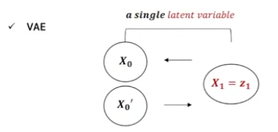
그 전에, VAE와 Diffusion model 사이의 차이를 잠깐 보면 아래와 같다.


3.1 Forward process and $L_T$
Forward process의 $\beta_t$는 VAE의 reparameterization trick으로 학습이 가능하지만 본 논문에서는 상수로 고정했다고 한다. 따라서 $L_T$는 학습되는 parameters를 가지지 않는다.
3.2 Reverse process and $L_{1:T-1}$
$L$의 $L_{t-1}$ 부분을 다룬다. $L_{t-1}$에서 reverse process $p_\theta(X_{t-1}|X_t)$은 KL divergence에 의해 forward process posterior $q(X_{t-1}|X_t, X_0)$을 근사하게 된다.
Forward process는 $q(X_{t-1}|X_t, X_0)$은 아래와 같은 gaussisan 형태로 $\beta_t$의 값에 따라 계산가능한 형태로 유도할 수 있다.

유도 과정은 아래의 자료를 참고했다.

Reverse process의 $p_\theta(X_{t-1}|X_t)=\mathcal{N}(X_{t-1};\mu_{\theta}(X_t, t), \Sigma_{\theta}(X_t, t))$을 봐보자.
첫째로, variance 부분인 $\Sigma_{\theta}(X_t, t) =\sigma^2 _tI$을 $\sigma^2_t=\beta_t$ 또는 $\sigma^2_t=\hat{\beta}_t=\frac{1-\bar{\alpha}_{t-1}}{ 1-\bar{\alpha}_{t}}\beta_t$ t와 같은 상수로 설정했고, 두 경우의 결과는 비슷했다고 한다.
둘째로, 앞서 variance 부분을 다음과 같이 $p_\theta(X_{t-1}|X_t)=\mathcal{N}(X_{t-1};\mu_{\theta}(X_t, t), \sigma^2_tI)$, 상수로 설정하였기 때문에 이제 $p_\theta(X_{t-1}|X_t)$의 mean인 $\mu_{\theta}(X_t, t)$만 구하면 된다.
이 부분은 단순하게 $q(X_{t-1}|X_t, X_0)$의 Mean, $\tilde{\mu}_{\theta}(X_t, t)$, 을 예측하는 신경망을 통해 구한다. 다음과 같이 $\tilde{\mu}_t$, $\mu_\theta$ 사이의 reconstruction error를 통해 모델을 학습시킬 수 있다. $\mu_\theta$를 딥러닝 모델로 이해하니 뒷 부분 수식을 이해하는 것이 조금 수훨했다.

논문에서는 이러한 수식을 representation하여 $\epsilon$에 대한 형태로 유도한다. (수식이 복잡해보인다... 하지만 오히려 단순해지는 과정이다.)

$X_t$는 $X_t(X_0, \epsilon)$로 표기하고, $X_t = \sqrt{\bar{\alpha}_t}X_0+\sqrt{1-\bar{\alpha}_t}\epsilon, \epsilon \sim \mathcal{N}(0,1)$을 사용하여 $X_0$를 $X_t$와 $\epsilon$의 형태로 바꾼다. 그리고 이를 앞서 Eq. (7)에서 유도한 $\tilde{\mu}_t(X_t, X_0)$에 대입하여 결과적으로 Eq. (10)의 꼴로 유도된다. (직접 해보지는 않았다;;)
결과적으로 Eq. (10)에 의하면 $X_t$가 주어졌을 때, 모델 $\mu_\theta$은 $\frac{1}{\sqrt{\alpha_t}}(X_t - \frac{\beta_t}{\sqrt{1-\bar{\alpha}_t}}\epsilon)$을 예측한다.
이때, $\frac{1}{\sqrt{\alpha_t}}(X_t - \frac{\beta_t}{\sqrt{1-\bar{\alpha}_t}}\epsilon)$에서 $\epsilon$을 제외한 나머지 값은 상수 값으로 주어지는 값이고, 모델에 의해 근사되는 부분은 노이즈인 $\epsilon$이다. 이를 $\epsilon_\theta(X_t, t)$로 표현하여 모델의 출력값은 $\mu_\theta(X_t, t) = \frac{1}{\sqrt{\alpha_t}}(X_t - \frac{\beta_t}{\sqrt{1-\bar{\alpha}_t}}\epsilon_\theta(X_t, t))$이고, 목적 함수 역시 아래와 같이 $\epsilon$에 대한 식 $dist(\epsilon, \epsilon_\theta)$으로 단순화 된다.

즉, reverse process에서 $X_{t-1} \sim p(X_{t-1}|X_t)$는 $X_{t-1} \sim \mathcal{N}(\frac{1}{\sqrt{\alpha_t}}(X_t - \frac{\beta_t}{\sqrt{1-\bar{\alpha}_t}}\epsilon_\theta(X_t, t)), \sigma^2_tI)$로 표현할 수 있다.
$X_{t-1}$을 샘플링한 값은 $\frac{1}{\sqrt{\alpha_t}}(X_t - \frac{\beta_t}{\sqrt{1-\bar{\alpha}_t}}\epsilon_\theta(X_t, t))+\sigma_tz, z \sim \mathcal{N}(0, I)$이 된다.
3.3 Data scaling, reverse process decoder, and $L_0$
$L_0$ term은 VAE의 reconstruction error와 같이 $X_0$와 $X_1$ 간의 복원 오차를 최소화하는 역할을 한다.
$L_2$ loss를 사용한다고 했을 때, $L_0 = \mathbb{E}_{q(\mathbf{x}_1|\mathbf{x}_0)} \left[ \|\mathbf{x}_0 - \mu_\theta (\mathbf{x}_1, 1) \|^2 \right]$과 같이 표현할 수 있을 것 같다.
3.4 Simplified training objective
본 논문에서는 앞서 유도한 목적함수를 더욱 단순화한다.

위의 수식에서 $t=1$인 경우, $L_0$와 일치한다. $t>1$인 경우, $L_{t-1}$의 unweighted version이 된다.
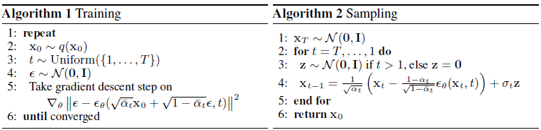
$L_{simple}$을 사용한 최종적인 학습 과정이 Algorithm 1에 나타난다.
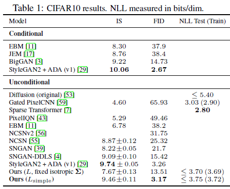
4. Experiments

참고 자료
- [모두팝] 생성모델무터 Diffusion까지 2회
- Blue collar Developer 블로그
- hanlyang0522.log 블로그 논문 리뷰
- LCY 블로그 논문 리뷰
- 유튜브 Diffusion Model 수학이 포함된 tutorial
- DSBA 연구실 논문리뷰
- Diffusion Model 설명 – 기초부터 응용까지


